d3-geo-projection
Extended geographic projections for d3-geo. See Command-Line Cartography for an introduction.
Installing
If you use npm, npm install d3-geo-projection. You can also download the latest release on GitHub. For vanilla HTML in modern browsers, import d3-geo-projection from Skypack:
<script type="module">

import {geoAitoff} from "https://cdn.skypack.dev/d3-geo-projection@4";

const projection = geoAitoff();

</script>
For legacy environments, you can load d3-geo-projection’s UMD bundle from an npm-based CDN such as jsDelivr; a d3 global is exported:
<script src="https://cdn.jsdelivr.net/npm/d3-array@3"></script>
<script src="https://cdn.jsdelivr.net/npm/d3-geo@3"></script>
<script src="https://cdn.jsdelivr.net/npm/d3-geo-projection@4"></script>
<script>

const projection = d3.geoAitoff();

</script>
API Reference
Projections
Note: projections tagged [d3-geo] are exported by d3-geo, not d3-geo-projection. These commonly-used projections are also included in the d3 default bundle.
# d3.geoAiry() · Source, Examples
# d3.geoAiryRaw(beta)
Airy’s minimum-error azimuthal projection.
# airy.radius([radius])
Defaults to 90°.
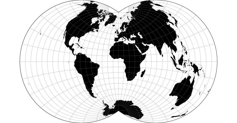
# d3.geoAitoff() · Source, Examples
# d3.geoAitoffRaw
The Aitoff projection.
# d3.geoAlbers() · Source [d3-geo]
Albers’ equal-area conic projection.
# d3.geoArmadillo() · Source, Examples
# d3.geoArmadilloRaw(phi0)
The armadillo projection. The default center assumes the default parallel of 20° and should be changed if a different parallel is used. Note: requires clipping to the sphere.
# armadillo.parallel([parallel])
Defaults to 20°.
# d3.geoAugust() · Source, Examples
# d3.geoAugustRaw
August’s epicycloidal conformal projection.
# d3.geoAzimuthalEqualArea() · Source [d3-geo], Examples
# d3.geoAzimuthalEqualAreaRaw
The Lambert azimuthal equal-area projection.
# d3.geoAzimuthalEquidistant() · Source [d3-geo], Examples
# d3.geoAzimuthalEquidistantRaw
The azimuthal equidistant projection.
# d3.geoBaker() · Source, Examples
# d3.geoBakerRaw
The Baker Dinomic projection.
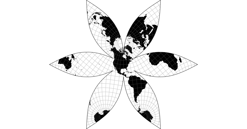
# d3.geoBerghaus() · Source, Examples
# d3.geoBerghausRaw(lobes)
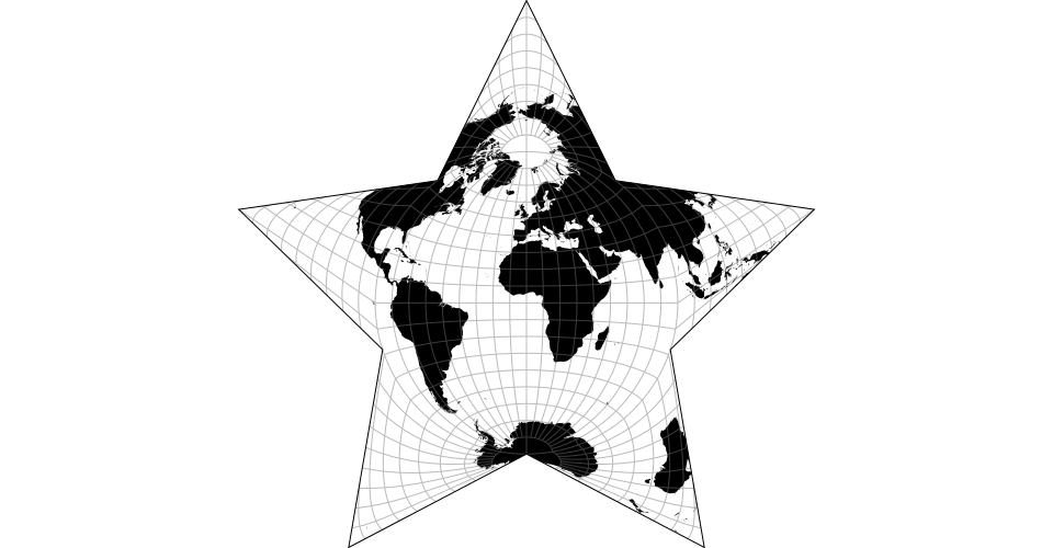
Berghaus’ star projection. The default center assumes the default lobe number of 5 and should be changed if a different number of lobes is used. Note: requires clipping to the sphere.
# berghaus.lobes([lobes]) · Source
If lobes is specified, sets the number of lobes in the resulting star, and returns this projection. If lobes is not specified, returns the current lobe number, which defaults to 5.
# d3.geoBertin1953() · Source
# d3.geoBertin1953Raw
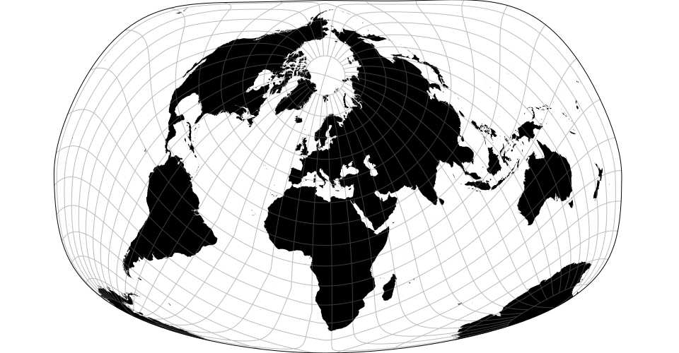
Jacques Bertin’s 1953 projection.
# d3.geoBoggs() · Source, Examples
# d3.geoBoggsRaw
The Boggs eumorphic projection. More commonly used in interrupted form.
# d3.geoBonne() · Source, Examples
# d3.geoBonneRaw(phi0)
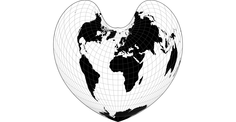
The Bonne pseudoconical equal-area projection. The Werner projection is a limiting form of the Bonne projection with a standard parallel at ±90°. The default center assumes the default parallel of 45° and should be changed if a different parallel is used.
# bonne.parallel([parallel])
Defaults to 45°.
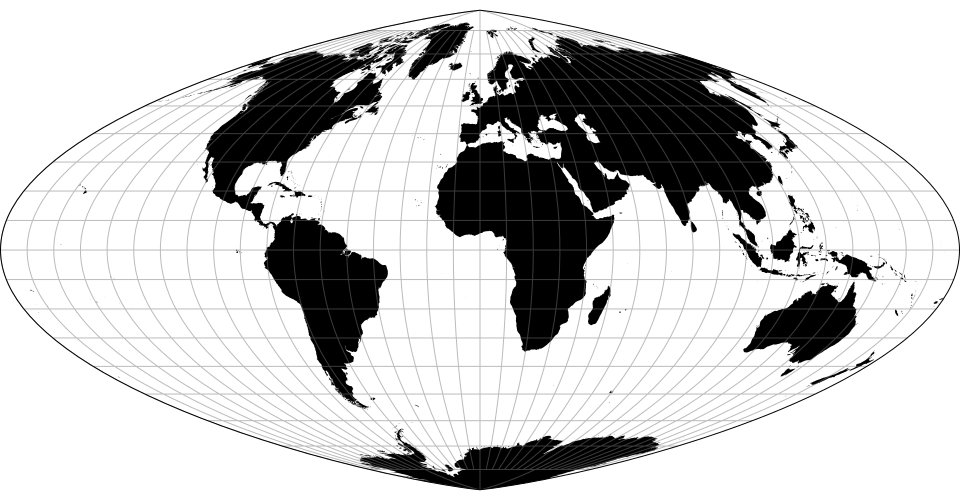
# d3.geoBottomley() · Source, Examples
# d3.geoBottomleyRaw(sinPsi)
The Bottomley projection “draws lines of latitude as concentric circular arcs, with arc lengths equal to their lengths on the globe, and placed symmetrically and equally spaced across the vertical central meridian.”
# bottomley.fraction([fraction])
Defaults to 0.5, corresponding to a sin(ψ) where ψ = π/6.
# d3.geoBromley() · Source, Examples
# d3.geoBromleyRaw
The Bromley projection is a rescaled Mollweide projection.
# d3.geoChamberlin(point0, point1, point2) · Source
# d3.geoChamberlinRaw(p0, p1, p2)
The Chamberlin trimetric projection. This method does not support projection.rotate: the three reference points implicitly determine a fixed rotation.
# d3.geoChamberlinAfrica() · Source
The Chamberlin projection for Africa using points [0°, 22°], [45°, 22°], [22.5°, -22°].
# d3.geoCollignon() · Source, Examples
# d3.geoCollignonRaw
The Collignon equal-area pseudocylindrical projection. This projection is used in the polar areas of the HEALPix projection.
# d3.geoConicConformal() · Source [d3-geo], Examples
# d3.geoConicConformalRaw
The Lambert conformal conic projection.
# d3.geoConicEqualArea() · Source [d3-geo], Examples
# d3.geoConicEqualAreaRaw
Albers’ conic equal-area projection.
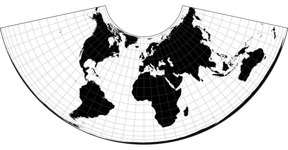
# d3.geoConicEquidistant() · Source [d3-geo], Examples
# d3.geoConicEquidistantRaw
The conic equidistant projection.
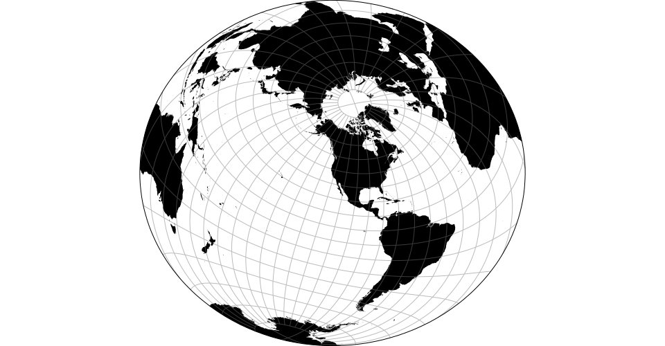
# d3.geoCraig() · Source, Examples
# d3.geoCraigRaw(phi)
The Craig retroazimuthal projection. Note: this projection tends to fold over itself if the standard parallel is non-zero; we have not yet implemented the necessary advanced clipping to avoid overlap.
# craig.parallel([parallel])
Defaults to 0°.
# d3.geoCraster() · Source, Examples
# d3.geoCrasterRaw
The Craster parabolic projection; also known as Putniņš P4.
# d3.geoCylindricalEqualArea() · Source, Examples
# d3.geoCylindricalEqualAreaRaw(phi0)
The cylindrical equal-area projection. Depending on the chosen parallel, this projection is also known as the Lambert cylindrical equal-area (0°), Behrmann (30°), Hobo–Dyer (37.5°), Gall–Peters (45°), Balthasart (50°) and Tobler world-in-a-square (~55.654°).
# cylindricalEqualArea.parallel([parallel])
Defaults to approximately 38.58°, fitting the world in a 960×500 rectangle.
# d3.geoCylindricalStereographic() · Source, Examples
# d3.geoCylindricalStereographicRaw(phi0)
The cylindrical stereographic projection. Depending on the chosen parallel, this projection is also known as Braun’s stereographic (0°) and Gall’s stereographic (45°).
# cylindricalStereographic.parallel([parallel])
Defaults to 0°.
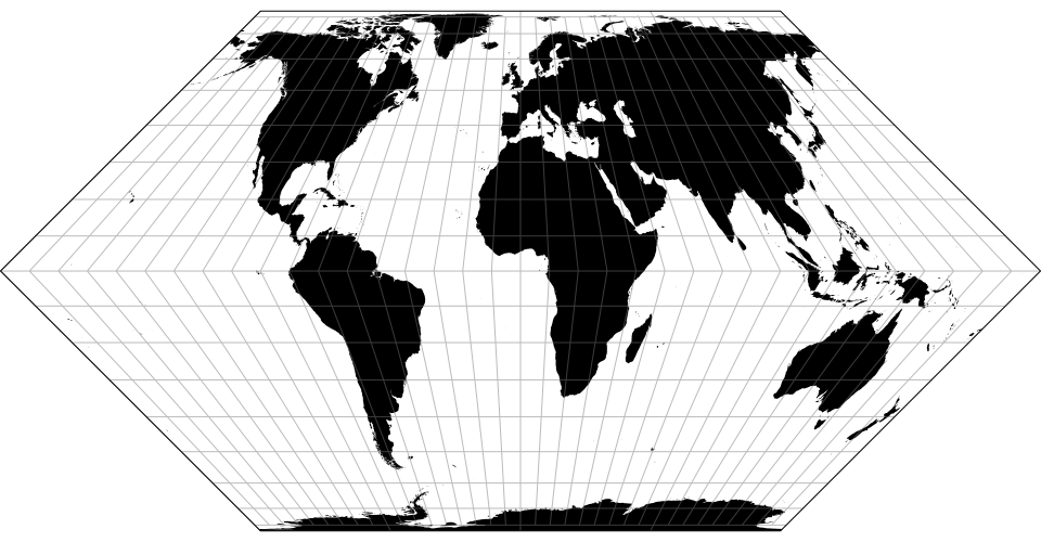
# d3.geoEckert1() · Source, Examples
# d3.geoEckert1Raw
The Eckert I projection.
# d3.geoEckert2() · Source, Examples
# d3.geoEckert2Raw
The Eckert II projection.
# d3.geoEckert3() · Source, Examples
# d3.geoEckert3Raw
The Eckert III projection.
# d3.geoEckert4() · Source, Examples
# d3.geoEckert4Raw

The Eckert IV projection.
# d3.geoEckert5() · Source, Examples
# d3.geoEckert5Raw
The Eckert V projection.
# d3.geoEckert6() · Source, Examples
# d3.geoEckert6Raw
The Eckert VI projection.
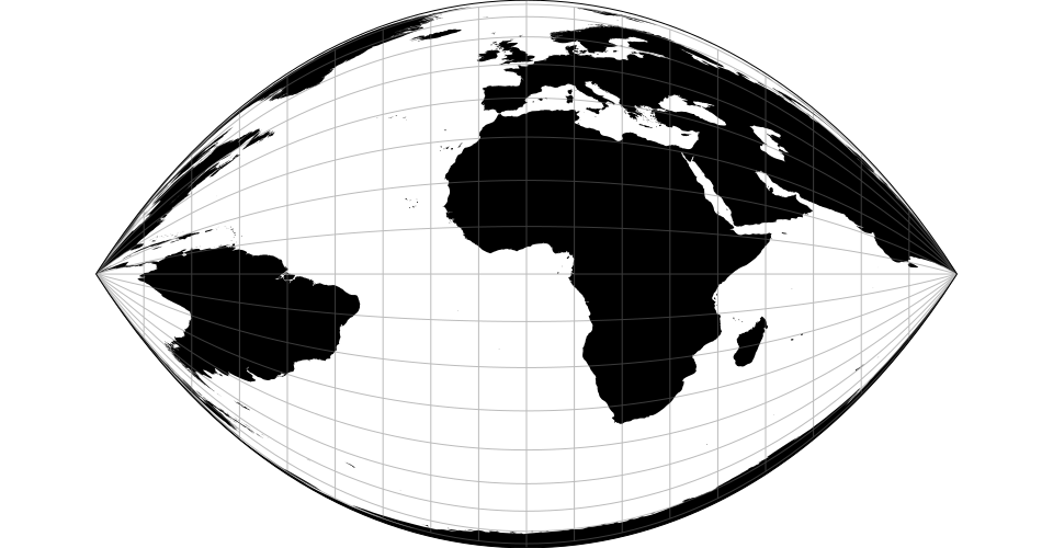
# d3.geoEisenlohr() · Source, Examples
# d3.geoEisenlohrRaw(lambda, phi)
The Eisenlohr conformal projection.
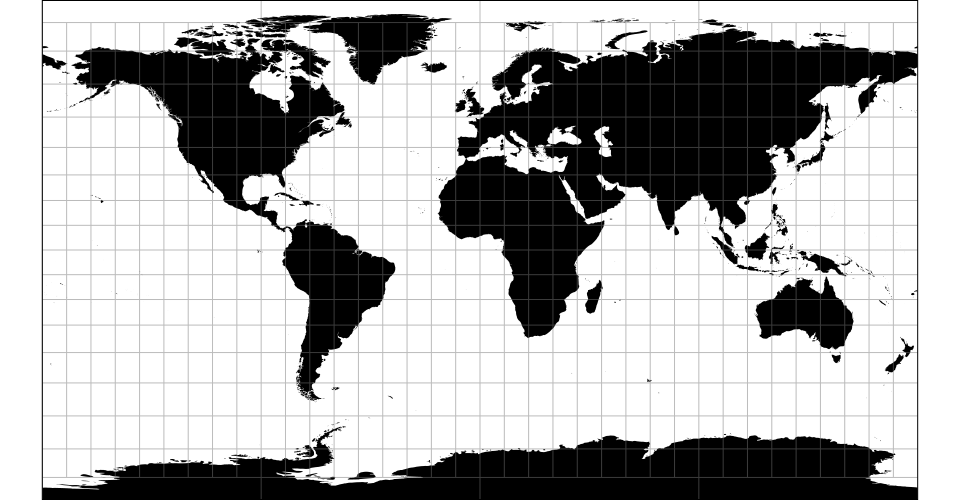
# d3.geoEquirectangular() · Source [d3-geo], Examples
# d3.geoEquirectangularRaw

The equirectangular (plate carrée) projection. The Cassini projection is the transverse aspect of the equirectangular projection.
# d3.geoFahey() · Source, Examples
# d3.geoFaheyRaw
The Fahey pseudocylindrical projection.
# d3.geoFoucaut() · Source, Examples
# d3.geoFoucautRaw
Foucaut’s stereographic equivalent projection.
# d3.geoFoucautSinusoidal() · Source, Examples
# d3.geoFoucautSinusoidalRaw

Foucaut’s sinusoidal projection, an equal-area average of the sinusoidal and Lambert’s cylindrical projections.
# foucautSinusoidal.alpha([alpha])
Relative weight of the cylindrical projection. Defaults to 0.5.
# d3.geoGilbert([type]) · Source, Examples
Gilbert’s two-world perspective projection. Wraps an instance of the specified projection type; if not specified, defaults to d3.geoOrthographic.
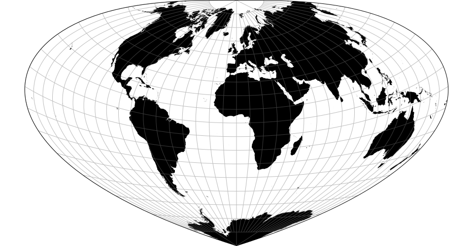
# d3.geoGingery() · Source, Examples
# d3.geoGingeryRaw(rho, lobes)
The U.S.-centric Gingery world projection, as inspired by Cram’s Air Age. Note: requires clipping to the sphere.
# gingery.radius([radius]) · Source
Defaults to 30°.
# gingery.lobes([lobes]) · Source
Defaults to 6.
# d3.geoGinzburg4() · Source, Examples
# d3.geoGinzburg4Raw
The Ginzburg IV projection.
# d3.geoGinzburg5() · Source, Examples
# d3.geoGinzburg5Raw
The Ginzburg V projection.
# d3.geoGinzburg6() · Source, Examples
# d3.geoGinzburg6Raw
The Ginzburg VI projection.
# d3.geoGinzburg8() · Source, Examples
# d3.geoGinzburg8Raw
The Ginzburg VIII projection.
# d3.geoGinzburg9() · Source, Examples
# d3.geoGinzburg9Raw
The Ginzburg IX projection.
# d3.geoGnomonic() · Source [d3-geo], Examples
# d3.geoGnomonicRaw
The gnomonic projection.
# d3.geoGringorten() · Source, Examples
# d3.geoGringortenRaw
The Gringorten square equal-area projection, rearranged to give each hemisphere an entire square.
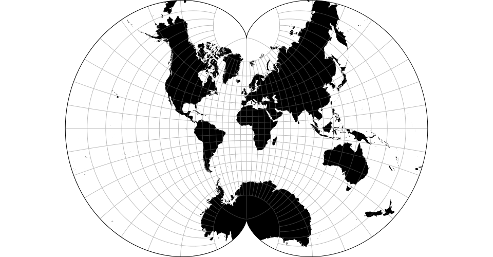
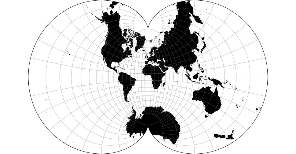
# d3.geoGuyou() · Source, Examples
# d3.geoGuyouRaw
The Guyou hemisphere-in-a-square projection. Peirce is credited with its quincuncial form.
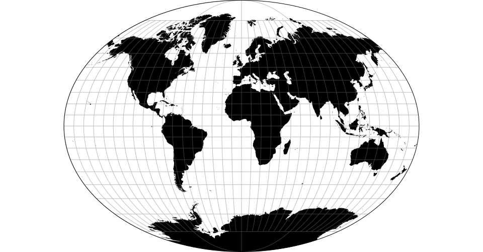
# d3.geoHammer() · Source, Examples
# d3.geoHammerRaw(A, B)
The Hammer projection. Depending the chosen coefficient and aspect, also known as Eckert–Greifendorff, quartic authalic, and Briesemeister.
# hammer.coefficient([coefficient]) · Source
Defaults to 2.
# d3.geoHammerRetroazimuthal() · Source, Examples
# d3.geoHammerRetroazimuthalRaw(phi0)
The Hammer retroazimuthal projection. Note: requires clipping to the sphere.
# hammerRetroazimuthal.parallel([parallel])
Defaults to 45°.
# d3.geoHealpix() · Source, Examples
# d3.geoHealpixRaw(lobes)
The HEALPix projection: a Hierarchical Equal Area isoLatitude Pixelisation of a 2-sphere. In this implementation, the parameter K is fixed at 3. Note: requires clipping to the sphere.
# healpix.lobes([lobes])
If lobes is specified, sets the number of lobes (the parameter H in the literature) and returns this projection. If lobes is not specified, returns the current lobe number, which defaults to 4.
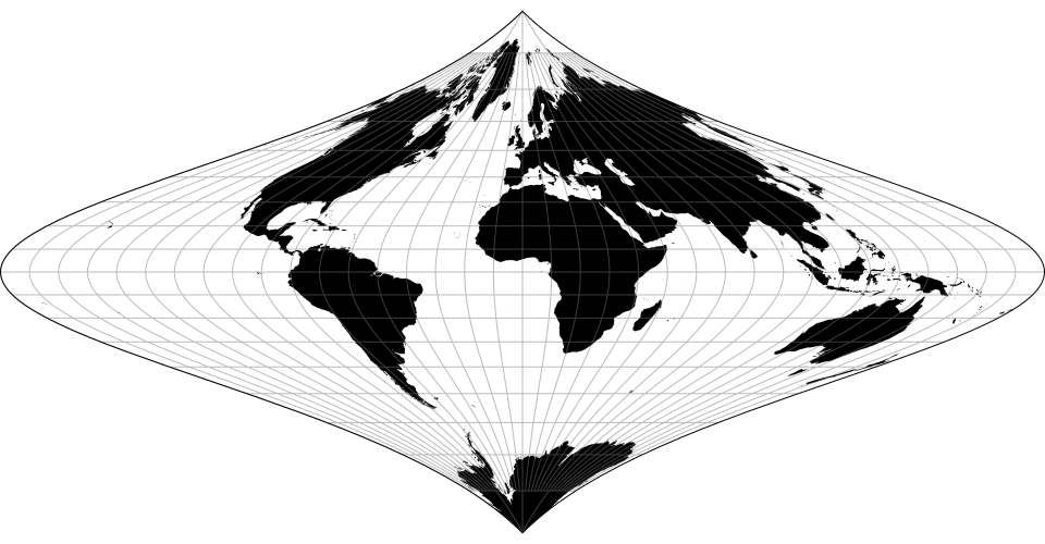
# d3.geoHill() · Source, Examples
# d3.geoHillRaw(K)
Hill eucyclic projection is pseudoconic and equal-area.
# hill.ratio([ratio])
Defaults to 1. With a ratio of 0, this projection becomes the Maurer No. 73. As it approaches ∞, the projection converges to the Eckert IV.
# d3.geoHomolosine() · Source, Examples
# d3.geoHomolosineRaw
The pseudocylindrical, equal-area Goode homolosine projection is normally presented in interrupted form.
# d3.geoHufnagel() · Source, Examples
# d3.geoHufnagelRaw
A customizable family of pseudocylindrical equal-area projections by Herbert Hufnagel.
# hufnagel.a([a])
# hufnagel.b([b])
# hufnagel.psiMax([psiMax])
# hufnagel.ratio([ratio])
# d3.geoHyperelliptical() · Source, Examples
# d3.geoHyperellipticalRaw
Waldo R. Tobler’s hyperelliptical is a family of equal-area pseudocylindrical projections. Parameters include k, the exponent of the superellipse (or Lamé curve) that defines the shape of the meridians (default k = 2.5); alpha, which governs the weight of the cylindrical projection that is averaged with the superellipse (default alpha = 0); and gamma, that shapes the aspect ratio (default: gamma = 1.183136).
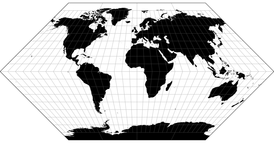
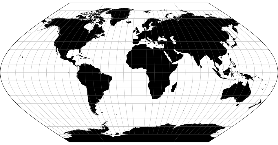
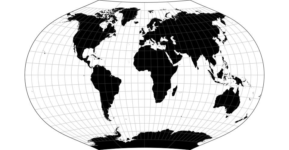
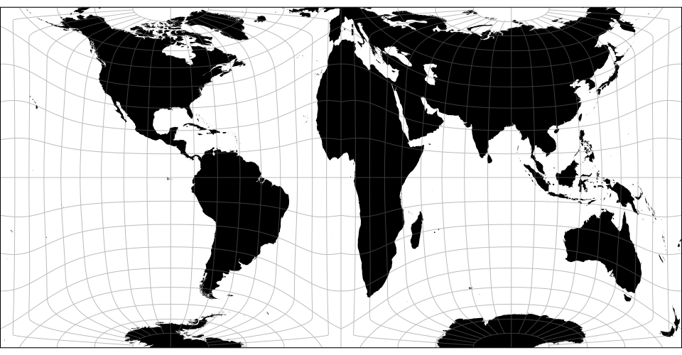
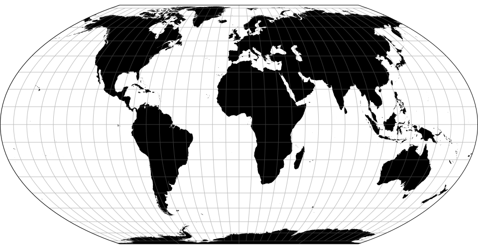
# d3.geoKavrayskiy7() · Source, Examples
# d3.geoKavrayskiy7Raw
The Kavrayskiy VII pseudocylindrical projection.
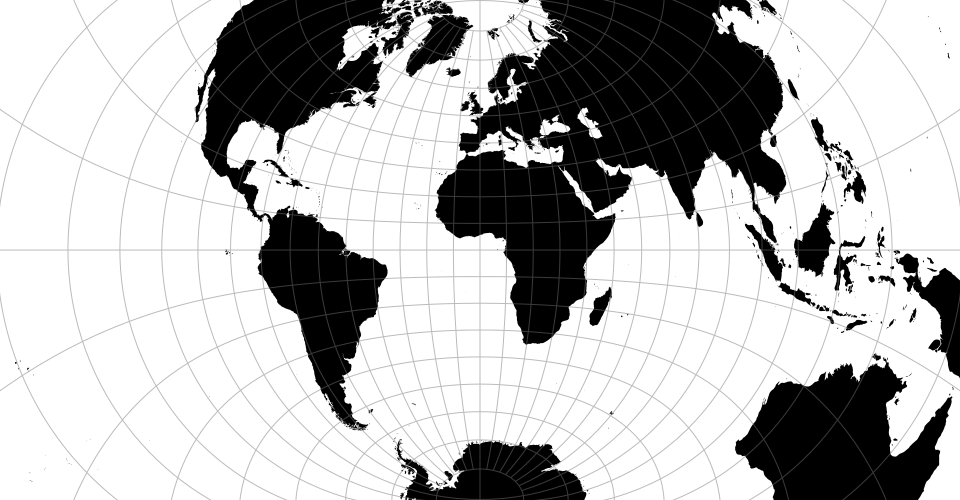
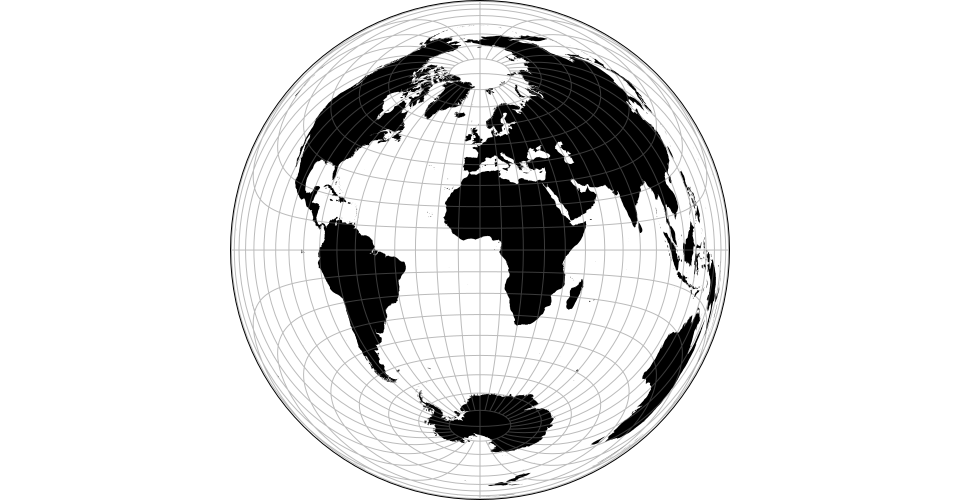
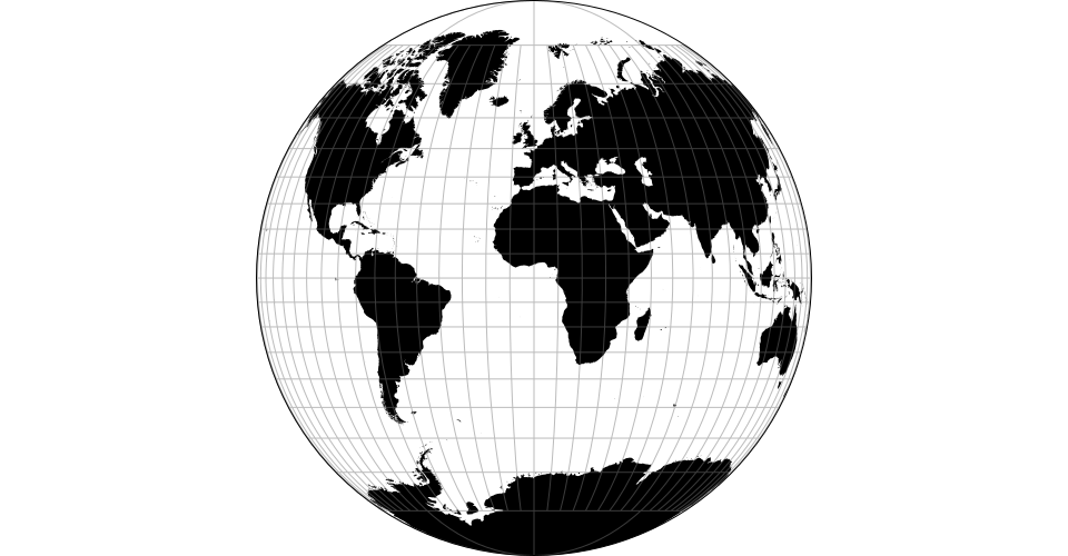
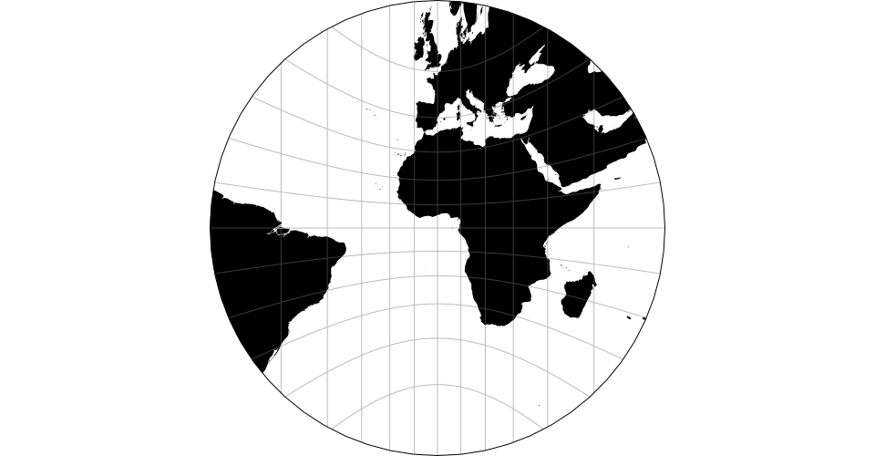
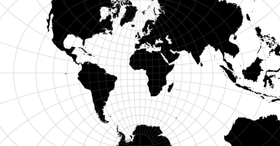
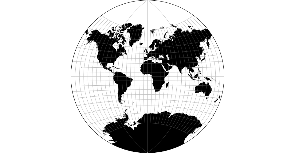
# d3.geoLagrange() · Source, Examples
# d3.geoLagrangeRaw(n)
The Lagrange conformal projection.
# lagrange.spacing([spacing])
Defaults to 0.5.
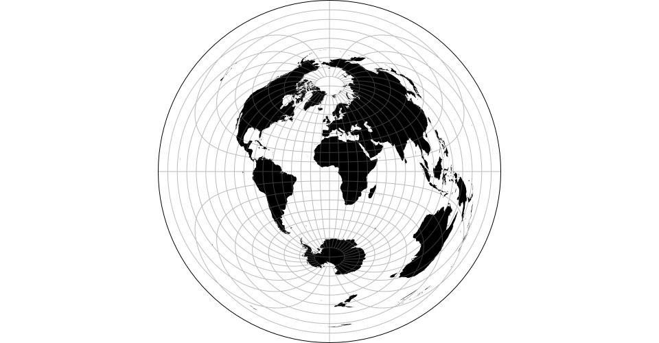
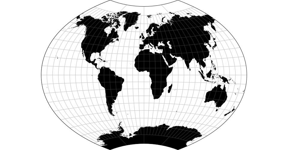
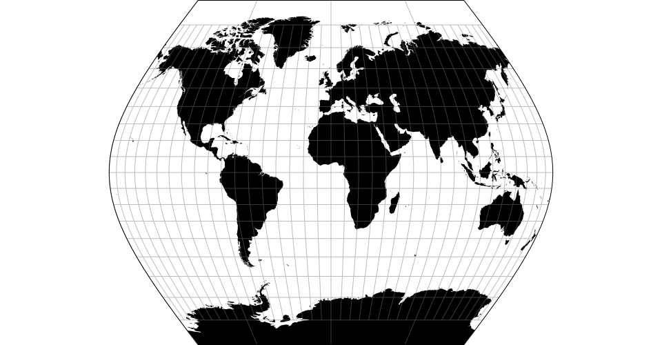
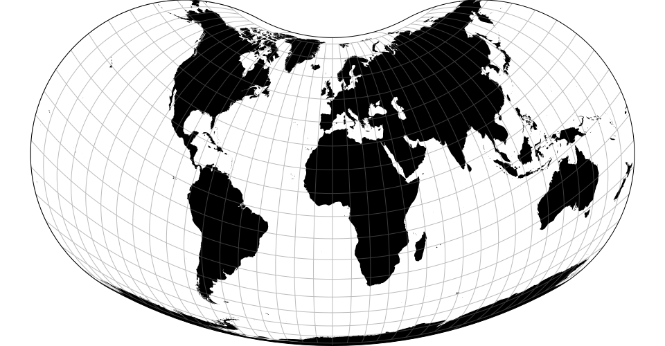
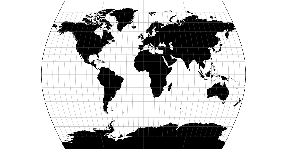
# d3.geoLarrivee() · Source, Examples
# d3.geoLarriveeRaw
The Larrivée projection.
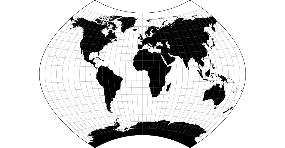
# d3.geoLaskowski() · Source, Examples
# d3.geoLaskowskiRaw
The Laskowski tri-optimal projection simultaneously minimizes distance, angular, and areal distortion.
# d3.geoLittrow() · Source, Examples
# d3.geoLittrowRaw
The Littrow projection is the only conformal retroazimuthal map projection. Typically clipped to the geographic extent [[-90°, -60°], [90°, 60°]].
# d3.geoLoximuthal() · Source, Examples
# d3.geoLoximuthalRaw(phi0)
The loximuthal projection is “characterized by the fact that loxodromes (rhumb lines) from one chosen central point (the intersection of the central meridian and central latitude) are shown as straight lines, correct in azimuth from the center, and are ‘true to scale’… It is neither an equal-area projection nor conformal.”
# loximuthal.parallel([parallel])
Defaults to 40°.
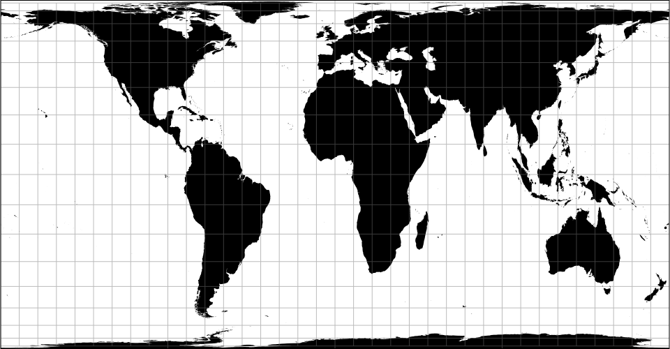
# d3.geoMercator() · Source [d3-geo], Examples
# d3.geoMercatorRaw
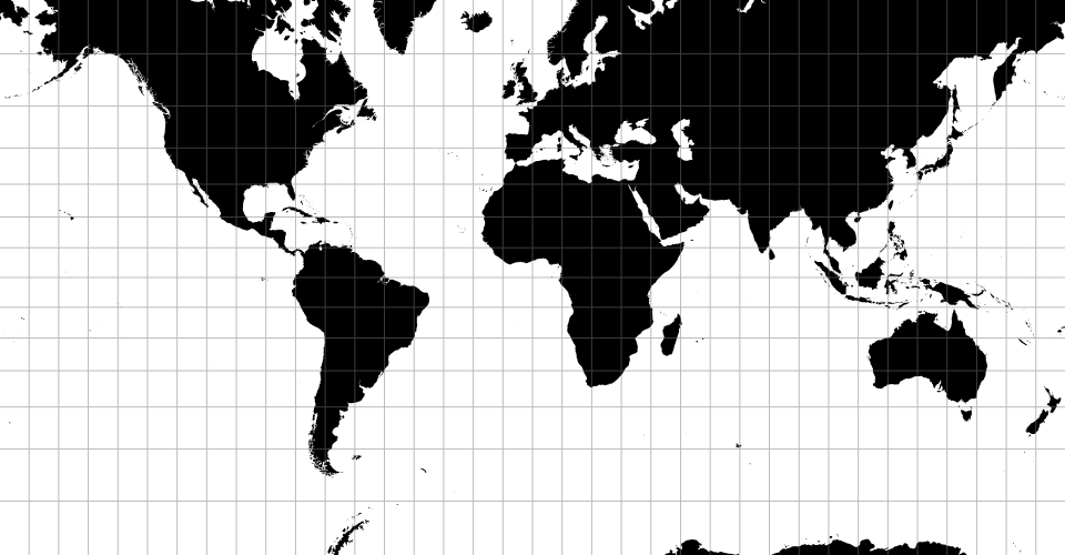
The spherical Mercator projection.
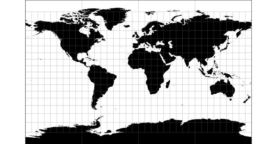
# d3.geoMiller() · Source, Examples
# d3.geoMillerRaw
The Miller cylindrical projection is a modified Mercator projection.
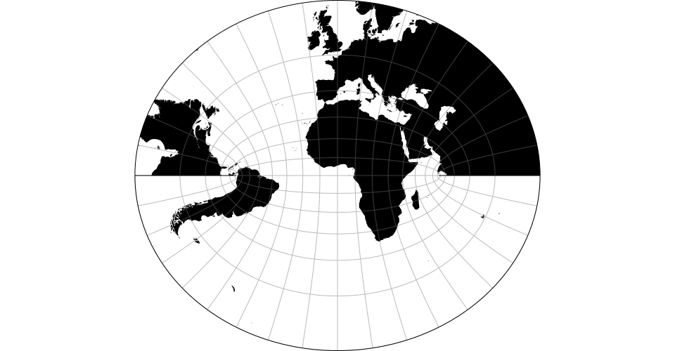
# d3.geoModifiedStereographic(coefficients, rotate) · Source
# d3.geoModifiedStereographicRaw(coefficients)
The family of modified stereographic projections. The default clip angle for these projections is 90°. These projections do not support projection.rotate: a fixed rotation is applied that is specific to the given coefficients.
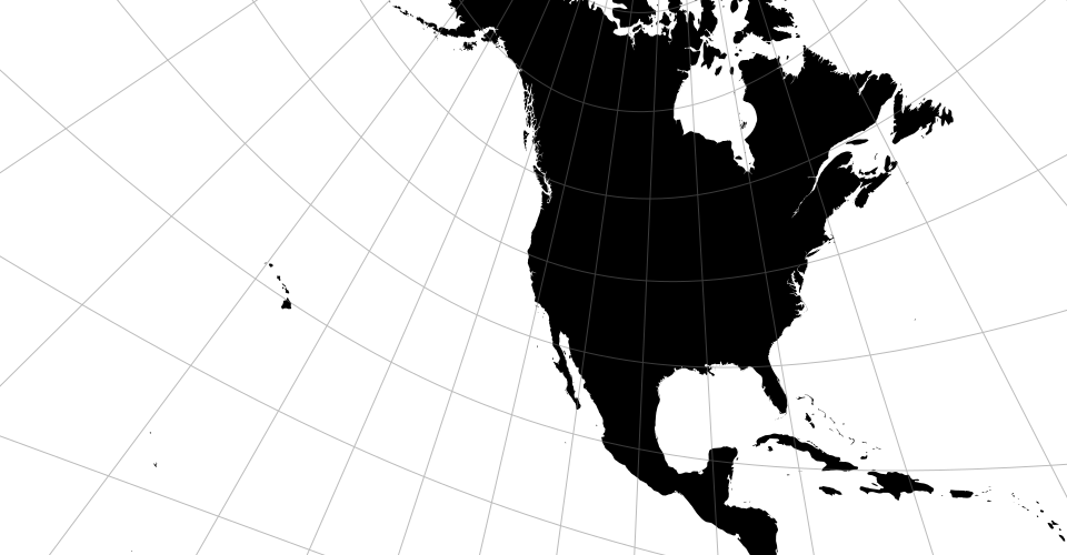
# d3.geoModifiedStereographicAlaska() · Source
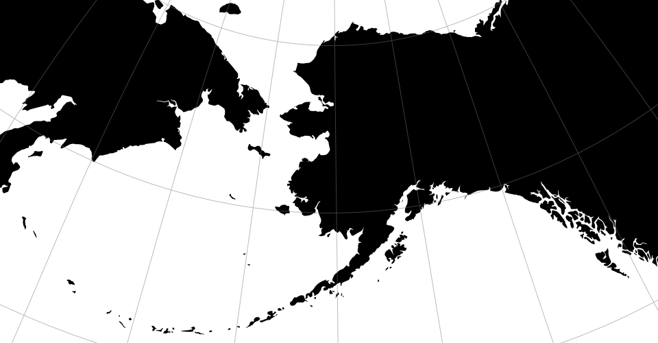
A modified stereographic projection for Alaska.
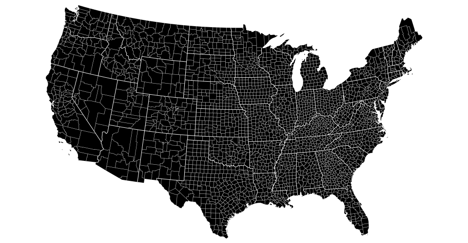
# d3.geoModifiedStereographicGs48() · Source
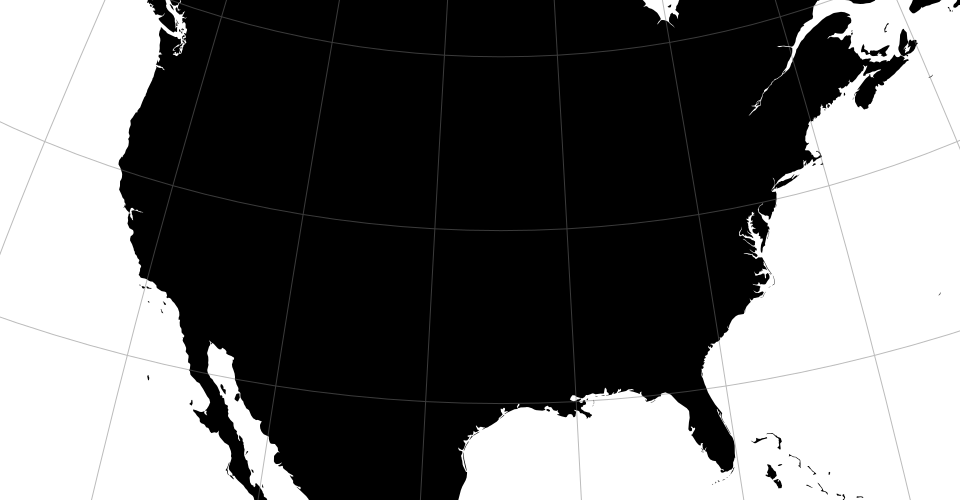
A modified stereographic projection for the conterminous United States.
# d3.geoModifiedStereographicGs50() · Source
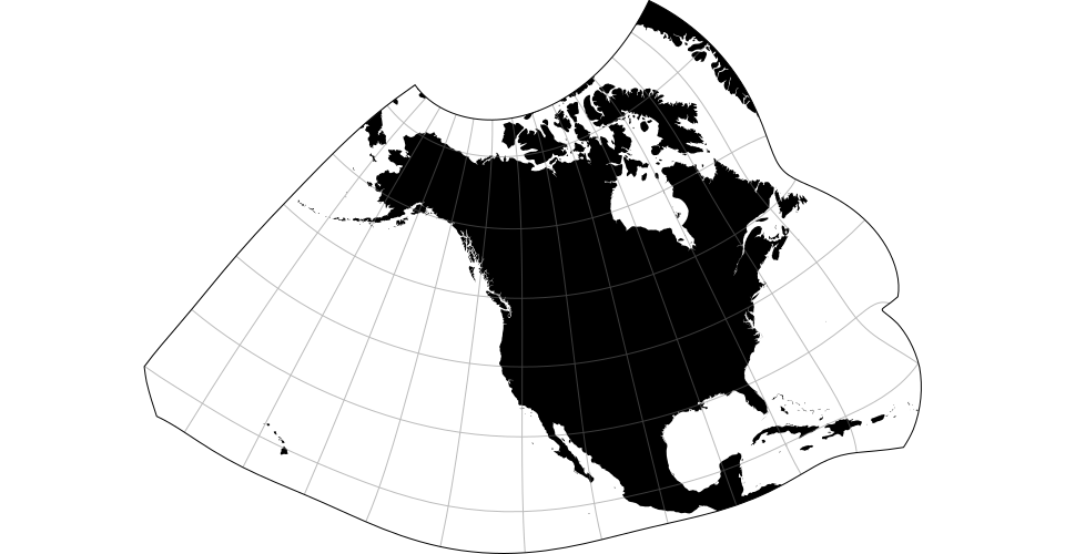
A modified stereographic projection for the United States including Alaska and Hawaii. Typically clipped to the geographic extent [[-180°, 15°], [-50°, 75°]].
# d3.geoModifiedStereographicMiller() · Source, Examples
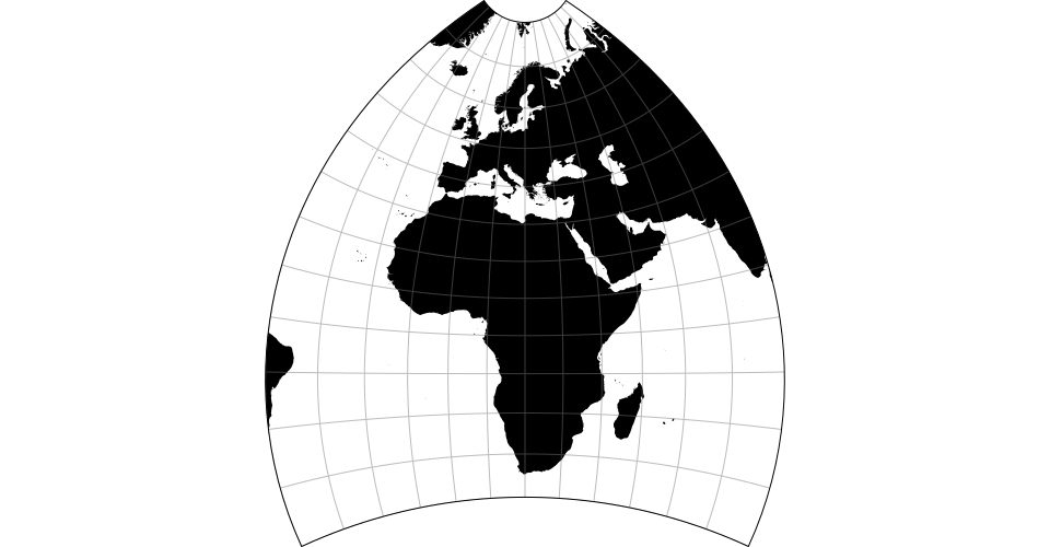
A modified stereographic projection for Europe and Africa. Typically clipped to the geographic extent [[-40°, -40°], [80°, 80°]].
# d3.geoModifiedStereographicLee() · Source, Examples
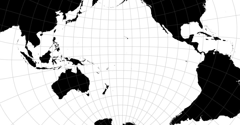
A modified stereographic projection for the Pacific ocean.
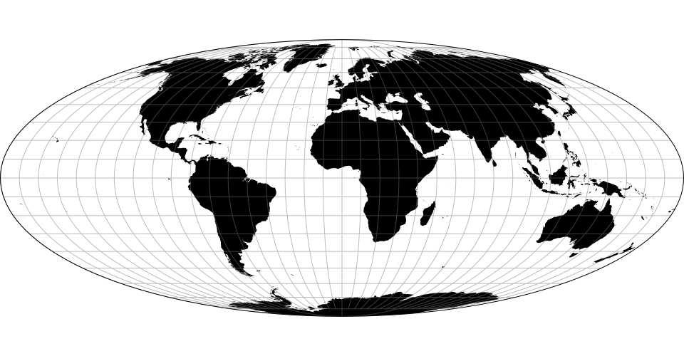
# d3.geoMollweide() · Source, Examples
# d3.geoMollweideRaw
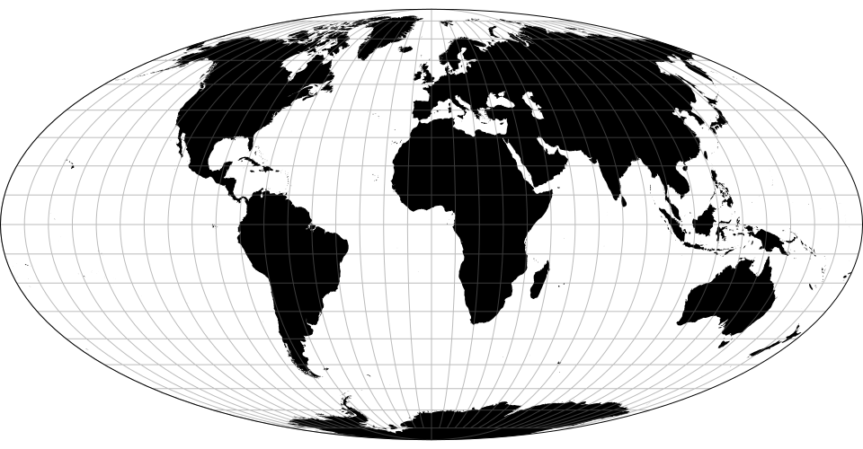
The equal-area, pseudocylindrical Mollweide projection. The oblique aspect is known as the Atlantis projection. Goode’s interrupted Mollweide is also widely known.
# d3.geoMtFlatPolarParabolic() · Source, Examples
# d3.geoMtFlatPolarParabolicRaw
The McBryde–Thomas flat-polar parabolic pseudocylindrical equal-area projection.
# d3.geoMtFlatPolarQuartic() · Source, Examples
# d3.geoMtFlatPolarQuarticRaw
The McBryde–Thomas flat-polar quartic pseudocylindrical equal-area projection.
# d3.geoMtFlatPolarSinusoidal() · Source, Examples
# d3.geoMtFlatPolarSinusoidalRaw
The McBryde–Thomas flat-polar sinusoidal equal-area projection.
# d3.geoNaturalEarth1() · Source [d3-geo], Examples
# d3.geoNaturalEarth1Raw
The Natural Earth projection.
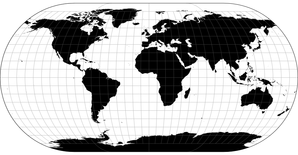
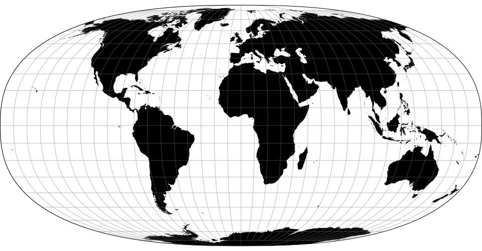
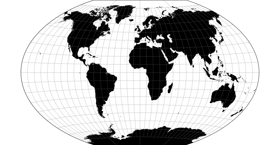
# d3.geoNaturalEarth2() · Source, Examples
# d3.geoNaturalEarth2Raw
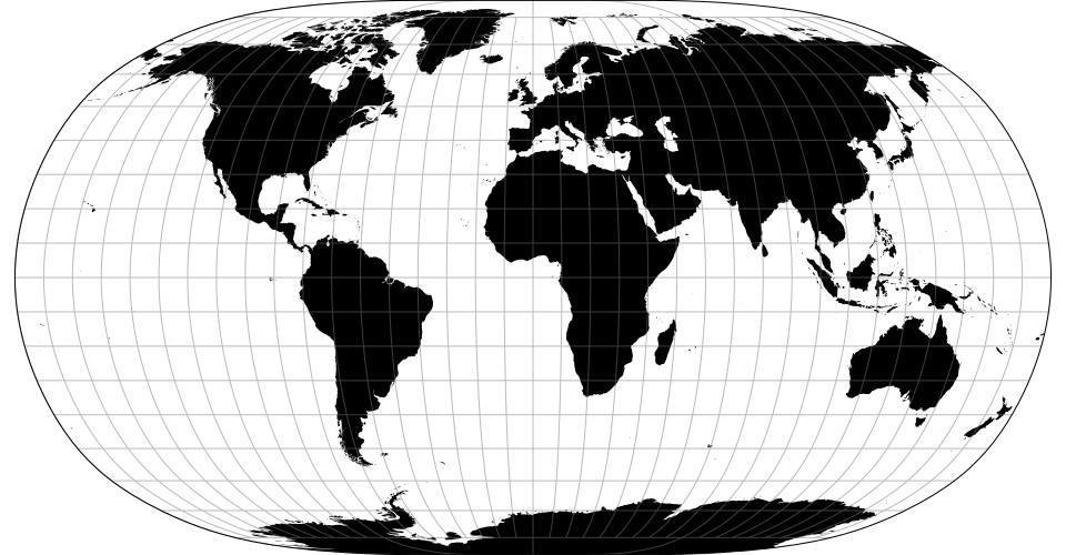
The Natural Earth II projection. Compared to Natural Earth, it is slightly taller and rounder.
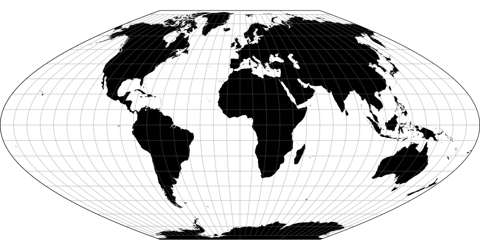
# d3.geoNellHammer() · Source, Examples
# d3.geoNellHammerRaw
The Nell–Hammer projection.
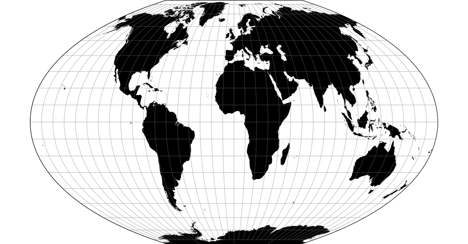
# d3.geoNicolosi() · Source, Examples
# d3.geoNicolosiRaw
The Nicolosi globular projection.
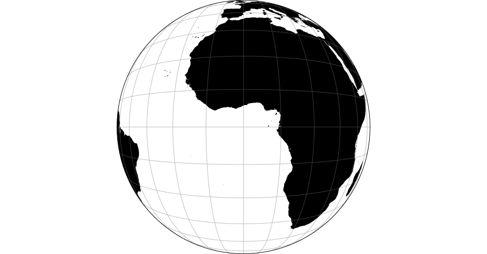
# d3.geoOrthographic() · Source [d3-geo], Examples
# d3.geoOrthographicRaw
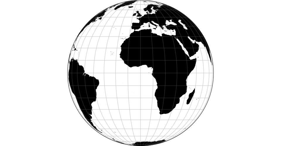
The orthographic projection.
# d3.geoPatterson() · Source, Examples
# d3.geoPattersonRaw
The Patterson cylindrical projection.
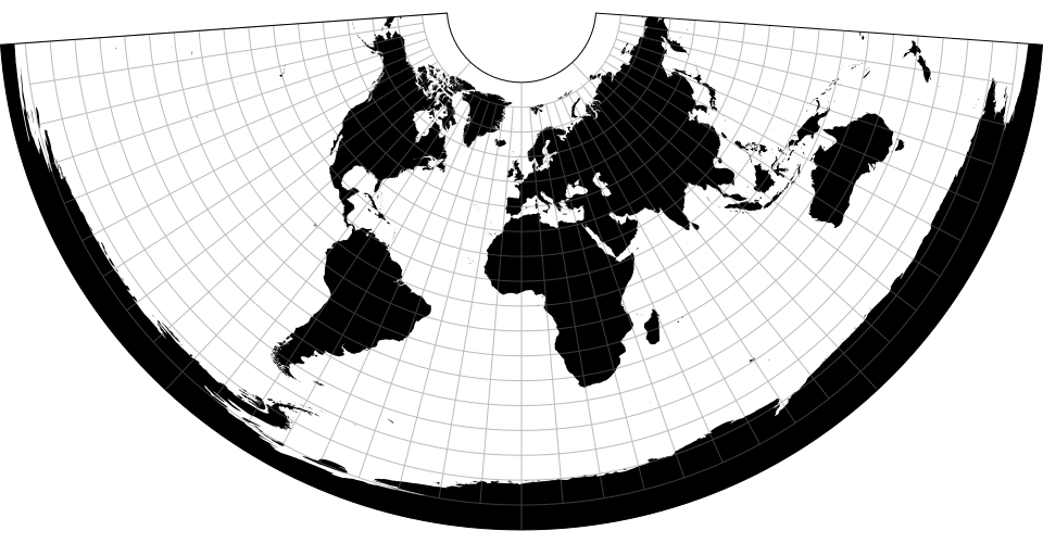
# d3.geoPolyconic() · Source, Examples
# d3.geoPolyconicRaw
The American polyconic projection.
# d3.geoRectangularPolyconic() · Source, Examples
# d3.geoRectangularPolyconicRaw(phi0)
The rectangular (War Office) polyconic projection.
# rectangularPolyconic.parallel([parallel])
Defaults to 0°.
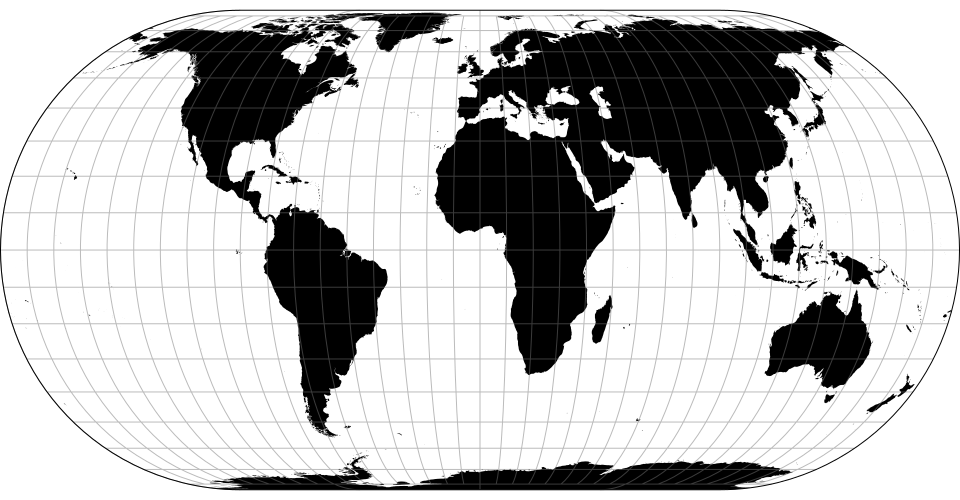
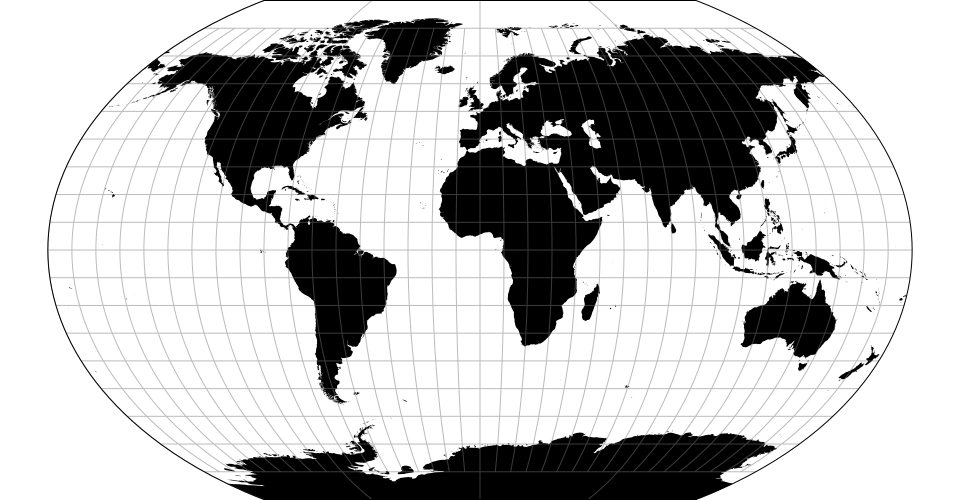
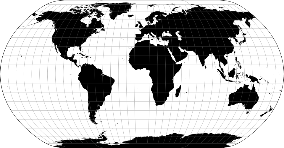
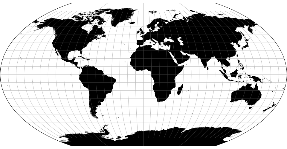
# d3.geoRobinson() · Source, Examples
# d3.geoRobinsonRaw
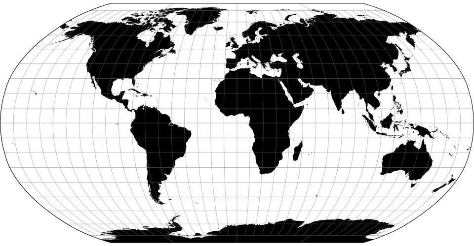
The Robinson projection.
# d3.geoSatellite() · Source, Examples
# d3.geoSatelliteRaw(P, omega)
The satellite (tilted perspective) projection.
# satellite.tilt([tilt])
Defaults to 0°.
# satellite.distance([distance])
Distance from the center of the sphere to the point of view, as a proportion of the sphere’s radius; defaults to 2.0. The recommended maximum clip angle for a given distance is acos(1 / distance) converted to degrees. If tilt is also applied, then more conservative clipping may be necessary. For exact clipping, the in-development geographic projection pipeline is needed; see the satellite explorer.
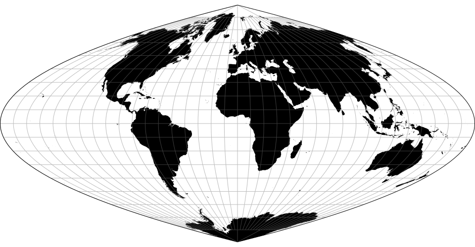
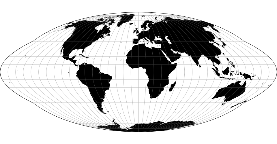
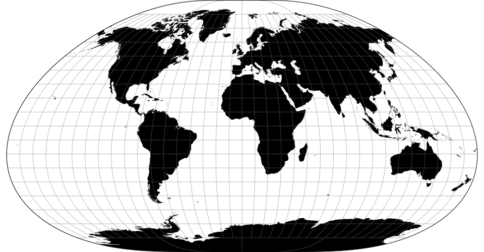
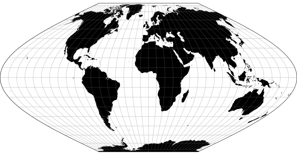
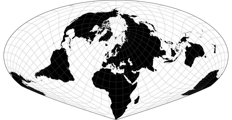
# d3.geoSinusoidal() · Source, Examples
# d3.geoSinusoidalRaw
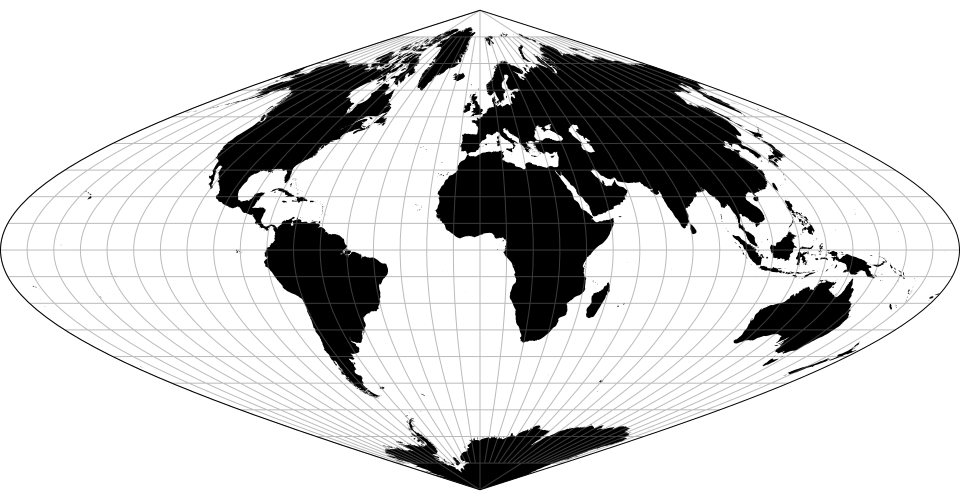
The sinusoidal projection.
# d3.geoSinuMollweide() · Source, Examples
# d3.geoSinuMollweideRaw
Allen K. Philbrick’s Sinu-Mollweide projection. See also the interrupted form.
# d3.geoStereographic() · Source [d3-geo], Examples
# d3.geoStereographicRaw
The stereographic projection.
# d3.geoTimes() · Source, Examples
# d3.geoTimesRaw
John Muir’s Times projection.
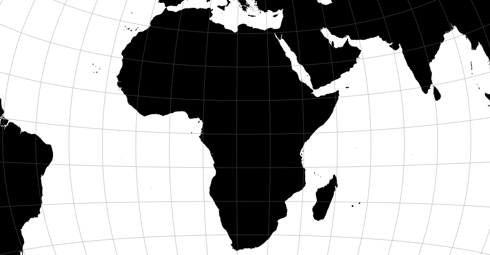
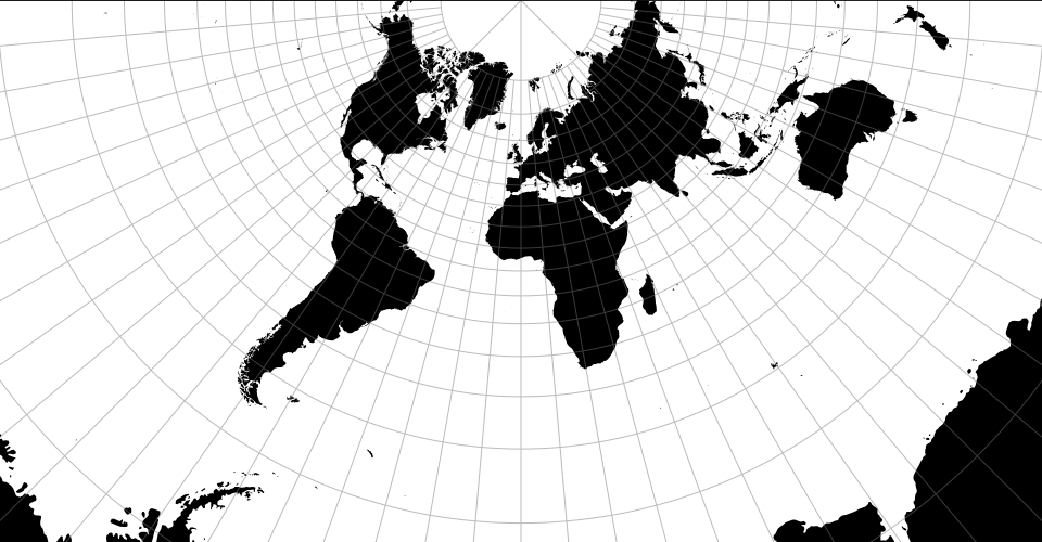
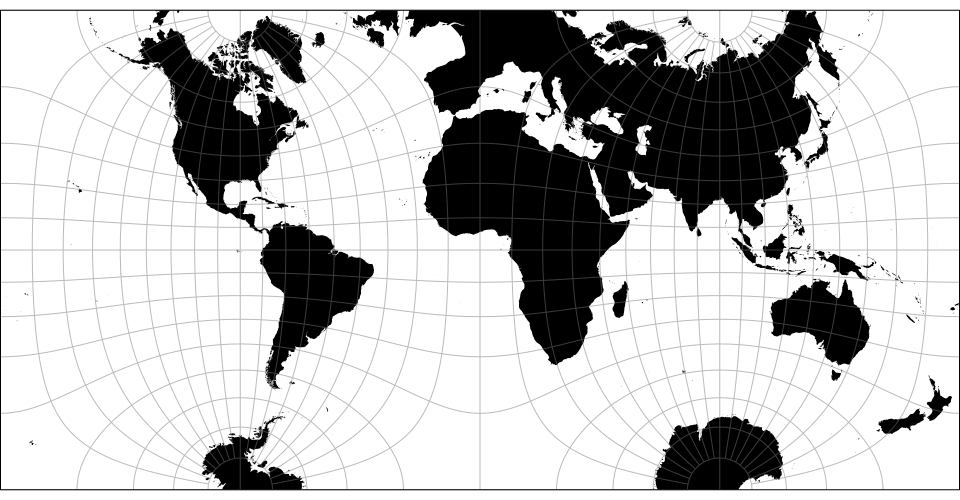
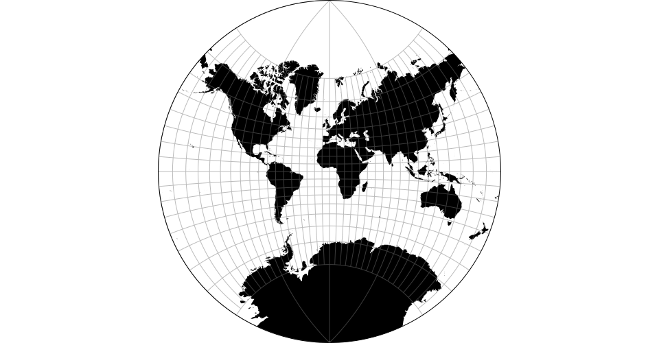
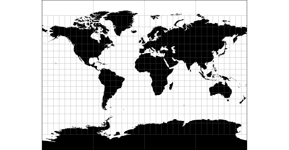
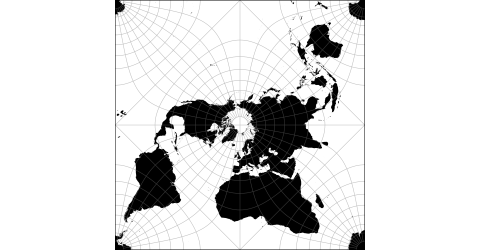
# d3.geoTransverseMercator() · Source [d3-geo], Examples
# d3.geoTransverseMercatorRaw
![]()
The transverse spherical Mercator projection.
# d3.geoTwoPointAzimuthal(point0, point1) · Source
# d3.geoTwoPointAzimuthalRaw(d)
The two-point azimuthal projection “shows correct azimuths (but not distances) from either of two points to any other point. [It can] be used to locate a ship at sea, given the exact location of two radio transmitters and the direction of the ship to the transmitters.” This projection does not support projection.rotate, as the rotation is fixed by the two given points.
# d3.geoTwoPointAzimuthalUsa() · Source
The two-point azimuthal projection with points [-158°, 21.5°] and [-77°, 39°], approximately representing Honolulu, HI and Washington, D.C.
# d3.geoTwoPointEquidistant(point0, point1) · Source
# d3.geoTwoPointEquidistantRaw(z0)
The two-point equidistant projection. This projection does not support projection.rotate, as the rotation is fixed by the two given points. Note: to show the whole Earth, this projection requires clipping to spherical polygons (example).
# d3.geoTwoPointEquidistantUsa() · Source
The two-point equidistant projection with points [-158°, 21.5°] and [-77°, 39°], approximately representing Honolulu, HI and Washington, D.C.
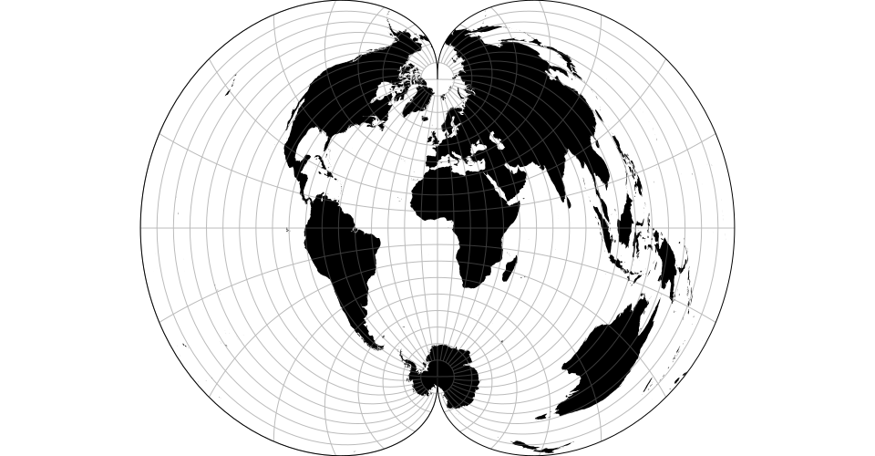
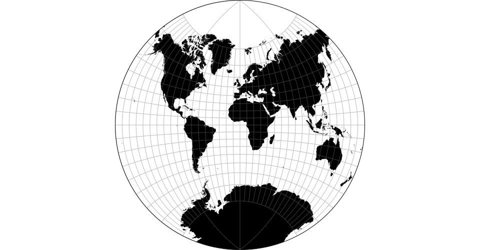
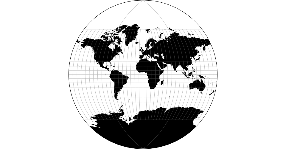
# d3.geoVanDerGrinten() · Source, Examples
# d3.geoVanDerGrintenRaw
The Van der Grinten projection.
# d3.geoVanDerGrinten2() · Source, Examples
# d3.geoVanDerGrinten2Raw
The Van der Grinten II projection.
# d3.geoVanDerGrinten3() · Source, Examples
# d3.geoVanDerGrinten3Raw
The Van der Grinten III projection.
# d3.geoVanDerGrinten4() · Source, Examples
# d3.geoVanDerGrinten4Raw
The Van der Grinten IV projection.
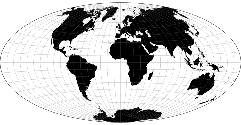
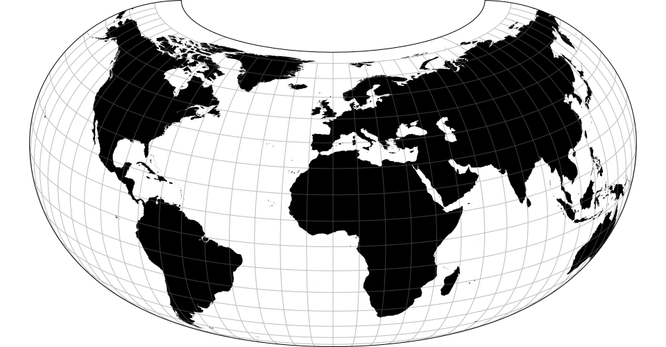
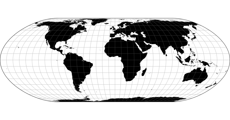
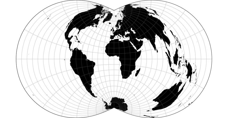
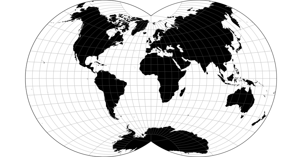
# d3.geoWagner() · Source, Examples
# d3.geoWagnerRaw
The Wagner projection is customizable: default values produce the Wagner VIII projection.
# wagner.poleline([poleline])
Defaults to 65°.
# wagner.parallels([parallels])
Defaults to 60°.
# wagner.inflation([inflation])
Defaults to 20.
# wagner.ratio([ratio])
Defaults to 200.
# d3.geoWagner4() · Source, Examples
# d3.geoWagner4Raw
The Wagner IV projection, also known as Putniṇš P2´.
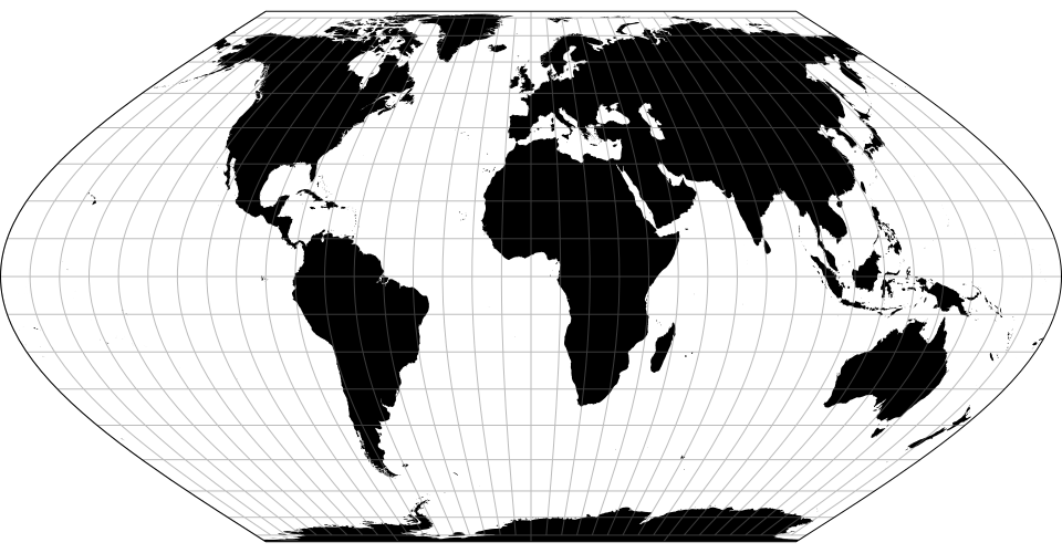
# d3.geoWagner6() · Source, Examples
# d3.geoWagner6Raw
The Wagner VI projection.
# d3.geoWagner7() · Source, Examples
The Wagner VII projection.
# d3.geoWiechel() · Source, Examples
# d3.geoWiechelRaw
The Wiechel projection.
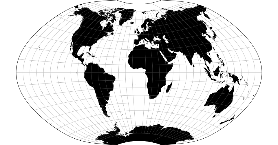
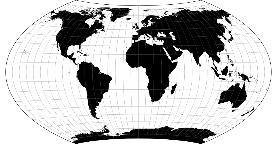
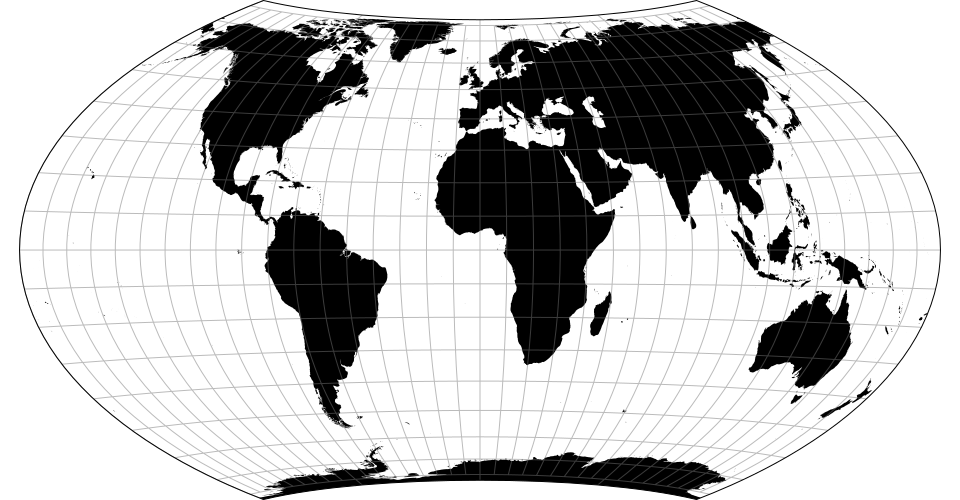
# d3.geoWinkel3() · Source, Examples
# d3.geoWinkel3Raw
The Winkel tripel projection.
Interrupted Projections
# d3.geoInterrupt(project, lobes) · Source, Examples
Defines a new interrupted projection for the specified raw projection function project and the specified array of lobes. The array lobes contains two elements representing the hemilobes for the northern hemisphere and the southern hemisphere, respectively. Each hemilobe is an array of triangles, with each triangle represented as three points (in degrees): the start, midpoint, and end. For example, the lobes in Goode’s interrupted homolosine projection are defined as:
[
  [
    [[-180,   0], [-100,  90], [ -40,   0]],
    [[ -40,   0], [  30,  90], [ 180,   0]]
  ],
  [
    [[-180,   0], [-160, -90], [-100,   0]],
    [[-100,   0], [ -60, -90], [ -20,   0]],
    [[ -20,   0], [  20, -90], [  80,   0]],
    [[  80,   0], [ 140, -90], [ 180,   0]]
  ]
]
Note: interrupted projections typically require clipping to the sphere.
# interrupted.lobes([lobes]) · Source
If lobes is specified, sets the new array of hemilobes and returns this projection; see d3.geoInterrupt for details on the format of the hemilobes array. If lobes is not specified, returns the current array of hemilobes.
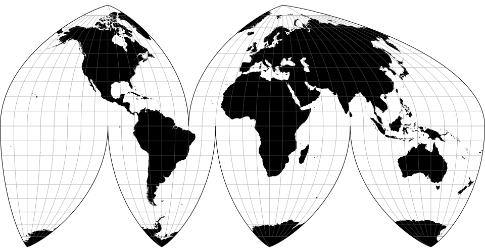
# d3.geoInterruptedHomolosine() · Source, Examples
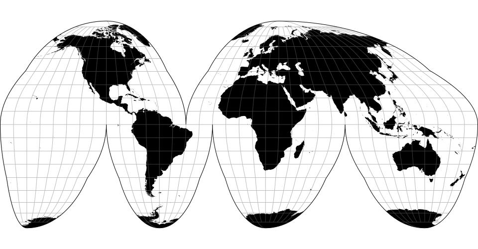
Goode’s interrupted homolosine projection. Its ocean-centric aspect is also well-known.
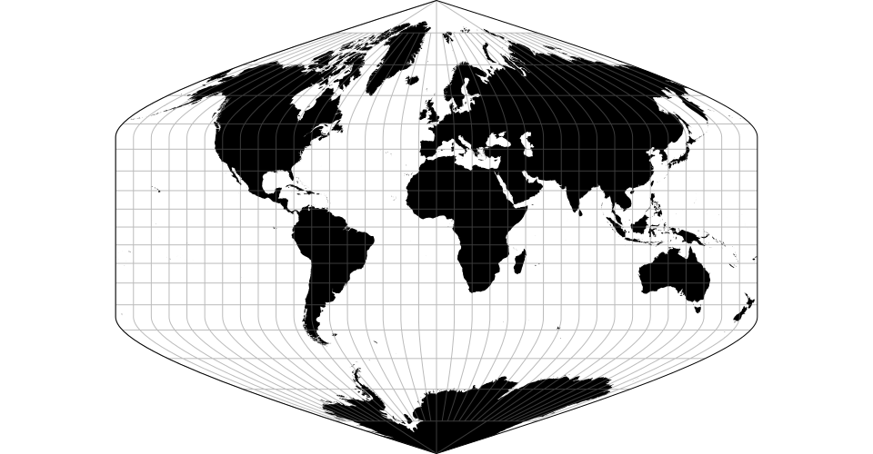
# d3.geoInterruptedSinusoidal() · Source, Examples
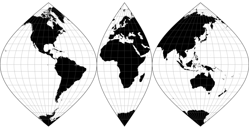
An interrupted sinusoidal projection with asymmetrical lobe boundaries that emphasize land masses over oceans, after the Swedish Nordisk Världs Atlas as reproduced by C.A. Furuti.
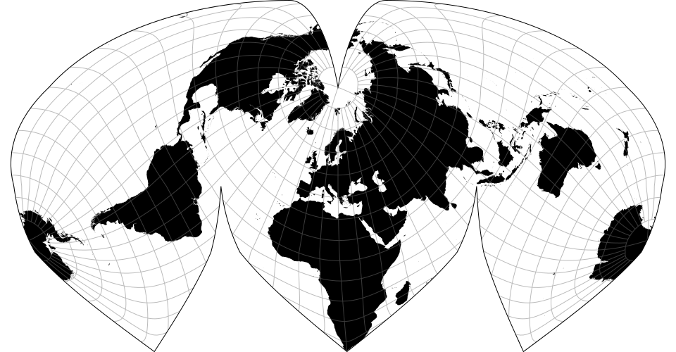
# d3.geoInterruptedBoggs() · Source, Examples
Bogg’s interrupted eumorphic projection.
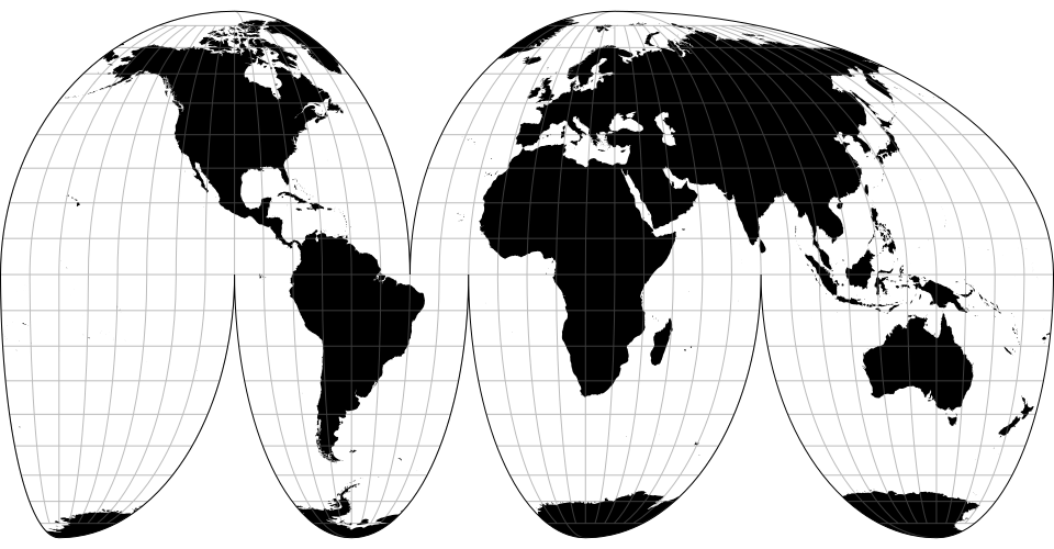
# d3.geoInterruptedSinuMollweide() · Source, Examples
Alan K. Philbrick’s interrupted sinu-Mollweide projection.
# d3.geoInterruptedMollweide() · Source, Examples
Goode’s interrupted Mollweide projection.
# d3.geoInterruptedMollweideHemispheres() · Source, Examples
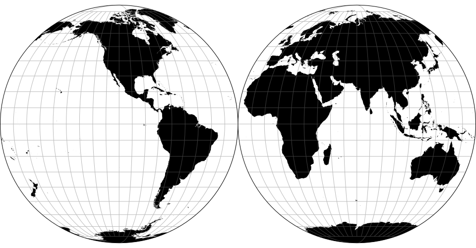
The Mollweide projection interrupted into two (equal-area) hemispheres.
# d3.geoInterruptedQuarticAuthalic() · Source, Examples
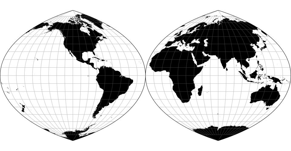
The quartic authalic projection interrupted into two hemispheres.
Polyhedral Projections
# d3.geoPolyhedral(root, face) · Source
Defines a new polyhedral projection. The root is a spanning tree of polygon face nodes; each node is assigned a node.transform matrix. The face function returns the appropriate node for a given lambda and phi in radians. Use projection.angle to set the orientation of the map (the default angle, -30°, might change in the next major version).
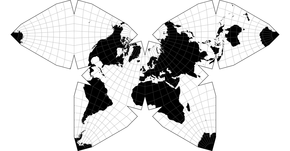
# d3.geoPolyhedralButterfly() · Source, Examples
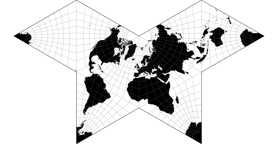
The gnomonic butterfly projection.
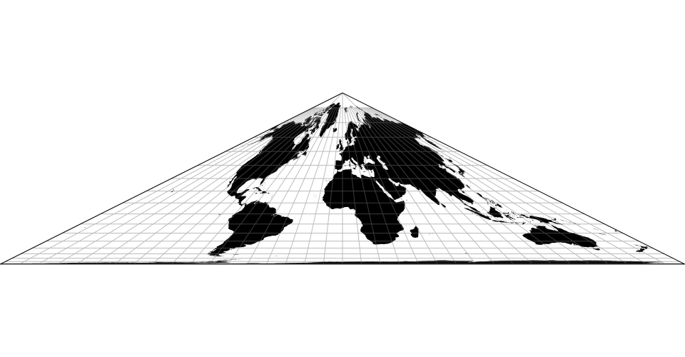
# d3.geoPolyhedralCollignon() · Source, Examples
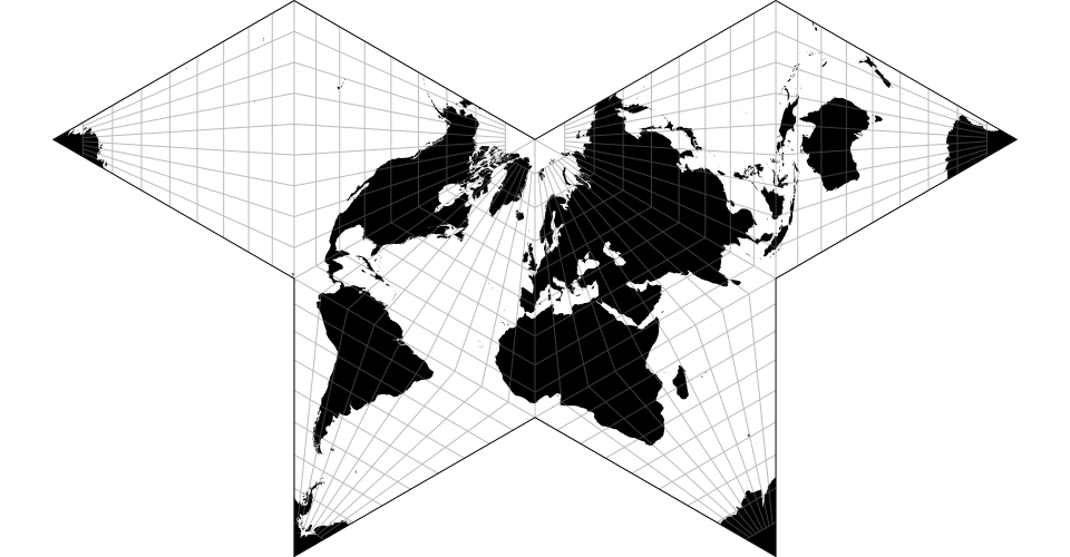
The Collignon butterfly projection.
# d3.geoPolyhedralWaterman() · Source, Examples
Steve Waterman’s butterfly projection.
Quincuncial Projections
# d3.geoQuincuncial(project) · Source
Defines a new quincuncial projection for the specified raw projection function project. The default rotation is [-90°, -90°, 45°] and the default clip angle is 180° - ε.
# d3.geoGringortenQuincuncial() · Source

The Gringorten square equal-area projection.
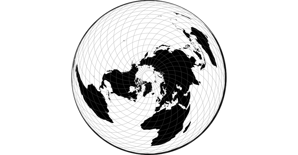
# d3.geoPeirceQuincuncial() · Source
The Peirce quincuncial projection is the quincuncial form of the Guyou projection.
Transformations
# d3.geoProject(object, projection) · Source
Projects the specified GeoJSON object using the specified projection, returning a shallow copy of the specified GeoJSON object with projected coordinates. Typically, the input coordinates are spherical and the output coordinates are planar, but the projection can also be an arbitrary geometric transformation.
See also geoproject.
# d3.geoStitch(object) · Source
Returns a shallow copy of the specified GeoJSON object, removing antimeridian and polar cuts, and replacing straight Cartesian line segments with geodesic segments. The input object must have coordinates in longitude and latitude in decimal degrees per RFC 7946. Antimeridian cutting, if needed, can then be re-applied after rotating to the desired projection aspect.
See also geostitch.
# d3.geoQuantize(object, digits) · Source
Returns a shallow copy of the specified GeoJSON object, rounding x and y coordinates according to number.toFixed. Typically this is done after projecting.
See also geoproject --precision and geo2svg --precision.
Command-Line Reference
geo2svg
# geo2svg [options…] [file] · Source
Converts the specified GeoJSON file to SVG. With --newline-delimited, each input feature is rendered as a separate path element; otherwise, a single path element is generated.
By default, the SVG’s fill is set to none and the stroke is set to black. The default point radius is 4.5. To override these values on a per-feature basis, the following GeoJSON feature properties will be propagated to attributes:
- fill
- fill-rule (or fillRule)
- fill-opacity (or fillOpacity)
- stroke
- stroke-width (or strokeWidth)
- stroke-linecap (or strokeLinecap)
- stroke-linejoin (or strokeLinejoin)
- stroke-miterlimit (or strokeMiterlimit)
- stroke-dasharray (or strokeDasharray)
- stroke-dashoffset (or strokeDashoffset)
- stroke-opacity (or strokeOpacity)
- point-radius (or pointRadius)
If the feature has an id, the path element will have a corresponding id attribute. If the feature has a title property, the path element will have a title element with the corresponding value. For an example of per-feature attributes, see this California population density map.
Note: per-feature attributes are most useful in conjunction with newline-delimited input, as otherwise the generated SVG only has a single path element. To set these properties dynamically, pass the input through ndjson-map.
Output usage information.
# geo2svg -V
# geo2svg --version
Output the version number.
# geo2svg -o file
# geo2svg --out file
Specify the output file name. Defaults to “-” for stdout.
# geo2svg -w value
# geo2svg --width value
Specify the output width. Defaults to 960.
# geo2svg -h value
# geo2svg --height value
Specify the output height. Defaults to 500.
# geo2svg -p value
# geo2svg --precision value
Reduce the precision for smaller output files. Defaults to six digits after the decimal point. See also d3.geoQuantize.
# geo2svg --fill value
Specify the default output fill color. Defaults to none.
# geo2svg --stroke value
Specify the default output stroke color. Defaults to black.
# geo2svg --r value
# geo2svg --radius value
Specify the default output point radius. Defaults to 4.5.
# geo2svg -n
# geo2svg --newline-delimited
Accept newline-delimited JSON as input, with one feature per line.
geograticule
# geograticule [options…] · Source
Generates a GeoJSON graticule. See also d3.geoGraticule.
# geograticule -h
# geograticule --help
Output usage information.
# geograticule -V
# geograticule --version
Output the version number.
# geograticule -o file
# geograticule --out file
Specify the output file name. Defaults to “-” for stdout.
# geograticule --extent value
Sets the graticule’s extent.
# geograticule --extent-minor value
Sets the graticule’s minor extent.
# geograticule --extent-major value
Sets the graticule’s major extent.
# geograticule --step value
Sets the graticule’s step.
# geograticule --step-minor value
Sets the graticule’s minor step.
# geograticule --step-major value
Sets the graticule’s major setp.
# geograticule --precision value
Sets the graticule’s precision.
geoproject
# geoproject [options…] projection [file] · Source
Projects the GeoJSON object in the specified input file using the specified projection, outputting a new GeoJSON object with projected coordinates. For example, to project standard WGS 84 input using d3.geoAlbersUsa:
geoproject 'd3.geoAlbersUsa()' us.json \
  > us-albers.json
For geometry that crosses the antimeridian or surrounds a pole, you will want to pass input through geostitch first:
geostitch world.json \
  | geoproject 'd3.geoMercator()' \
  > world-mercator.json
Typically, the input coordinates are spherical and the output coordinates are planar, but the projection can also be an arbitrary geometric transformation. For example, to invert the y-axis of a standard spatial reference system such as California Albers (EPSG:3310) and fit it to a 960×500 viewport:
shp2json planar.shp \
  | geoproject 'd3.geoIdentity().reflectY(true).fitSize([960, 500], d)' \
  > planar.json
See also d3.geoProject and d3.geoIdentity.
# geoproject -h
# geoproject --help
Output usage information.
# geoproject -V
# geoproject --version
Output the version number.
# geoproject -o file
# geoproject --out file
Specify the output file name. Defaults to “-” for stdout.
# geoproject -p value
# geoproject --precision value
Reduce the precision for smaller output files. See also d3.geoQuantize.
# geoproject -n
# geoproject --newline-delimited
Accept newline-delimited JSON as input, with one feature per line, and generate newline-delimited JSON as output.
# geoproject -r [name=]value
# geoproject --require [name=]value
Requires the specified module, making it available for use in any expressions used by this command. The loaded module is available as the symbol name. If name is not specified, it defaults to module. (If module is not a valid identifier, you must specify a name.) For example, to reproject the world on the Airocean projection:
geoproject --require d3=d3-geo-polygon 'd3.geoAirocean()' world.geojsonThe required module is resolved relative to the current working directory. If the module is not found during normal resolution, the global npm root is also searched, allowing you to require globally-installed modules from the command line.
Multiple modules can be required by repeating this option.
geoquantize
# geoquantize [options…] [file] · Source
Reads the GeoJSON object from the specified input file and outputs a new GeoJSON object with coordinates reduced to precision. Same options as geoproject.
geoquantize us.json --precision 3 \
  > us-quantized.json
geostitch
# geostitch [options…] [file] · Source
Stitches the GeoJSON object in the specified input file, removing antimeridian and polar cuts, and replacing straight Cartesian line segments with geodesic segments. The input object must have coordinates in longitude and latitude in decimal degrees per RFC 7946. Antimeridian cutting, if needed, can then be re-applied after rotating to the desired projection aspect.
See geoproject for an example. See also d3.geoStitch.
# geostitch -h
# geostitch --help
Output usage information.
# geostitch -V
# geostitch --version
Output the version number.
# geostitch -o file
# geostitch --out file
Specify the output file name. Defaults to “-” for stdout.
# geostitch -n
# geostitch --newline-delimited
Accept newline-delimited JSON as input, with one feature per line, and generate newline-delimited JSON as output.